Use hidden measures and members from #PowerBI dataset in an Excel Pivot table

When you connect to a Power BI Dataset from Power BI desktop you might have noticed that you can see and use hidden measures and columns in the dataset.

But the hidden fields cannot be seen if you browse the dataset in Excel.

But that does not mean that you cannot use the fields in Excel – and here is how you can do it.

Using VBA

You can use VBA by creating a macro

The code will add the field AddressLine1 from the DImReseller dimension as a Rowfield if the active cell contains a pivotable.

Sub AddField()
    Dim pv As PivotTable
        Set pv = ActiveCell.PivotTable
        pv.CubeFields("[DimReseller].[AddressLine1]").Orientation = xlRowField
End Sub

If you want to add a measure/value to the pivotable you need to set change the Orientation property to xlDataFields

This means that we now have added two hidden fields from the dataset

Add hidden measures using OLAP Tools

You can also add hidden measures using the OLAP Tools and MDX Calculated Measure

Simply create a new calculated measure by referencing the hidden measure in the MDX

This will add a calculated Measure to the measure group you selected

And you can add that to your pivotable

Referencing hidden items using CUBE functions

Notice that you can also reference the hidden measures using CUBE functions

Simply specify the name of the measure as the member expression in this case as “[Measures].[Sales Profit]”

You can also refer to members from hidden fields using the CUBEMEMBER functions

Hope this can help you too.

Power On!

Short Cut Keys– that every Excel user should know

Here is a list of short cut keys that I almost use every time I work in Excel.

The short cut keys works in the English version of Excel – localized version may use other keys.

CTRL + ‘ – copies the content of the cell above and enter edit state of the cell – very handy when creating almost the same formula as the cell above

F4 – when you are editing a cell reference in the formula bar the key cycles through the absolute and relative for column ref and row ref

CTRL+ _ (underscore) – removes any border around the selected cells

CTRL + ENTER – when a range or multiple cells is selected and you press CTRL + ENTER when you input values or formulas the input will be inserted in your entire selection

CTRL + F1 – Hide the Ribbon

CTRL + 1 – Open the format cells dialog

Hope these can help you too – if you have other favourites please let me know in the comments below.

 

Excel Tip – Easy way to remove all value fields from your pivottable #excel

If you want to remove all your value fields from your pivot table – you should not do this by removing the fields one by one.

Instead of removing each field from the Values area in the PivotTable Fields action pane one by one – simply remove the Values field in the column or rows area.

Instead of removing each field from the Values area in the PivotTable Fields action pane one by one – simply remove the Values field in the column or rows area.

That will remove all your value fields from the pivottable.

Hope this little trick can help you too.

Visualize the danish mobile network history & coverage using #PowerQuery and #PowerMap – #powerbi

A lot of public datasets is available via this site http://datahub.virk.dk/data/search – currently only in Danish.

One of the datasets contains information about the location of all the antennas in Denmark – http://mastedatabasen.dk/Viskort/ContentPages/DataFraDatabasen.aspx?callingapp=mastedb – and it has an excellent API that enables you to extract data about the antennas.

Here is how you can extract the data using Power Query and then visualize it in Power Map using Excel 2016 – you can do the same in Excel 2013 but I was playing around with Excel 2016.

First I select the

And paste in this query – which will return all the antennas in Denmark – it will return about 27.000 but I set the Max to 100.000

http://mastedatabasen.dk/Master/antenner.json?maxantal=100000

Click the To Table in the ribbon – accept the default and then Expand the column – then you have the data

The rest of the steps is deleting unwanted columns and renaming the fields and changing the established column to a date.

All the steps is as follows

let

Source = Json.Document(Web.Contents(“http://mastedatabasen.dk/Master/antenner.json?maxantal=100000”)),

#”Converted to Table” = Table.FromList(Source, Splitter.SplitByNothing(), null, null, ExtraValues.Error),

#”Expanded Column1″ = Table.ExpandRecordColumn(#”Converted to Table”, “Column1”, {“vejnavn”, “husnr”, “postnummer”, “kommune”, “idriftsaettelsesdato”, “forventet_idriftsaettelsesdato”, “etrs89koordinat”, “wgs84koordinat”, “tjenesteart”, “teknologi”, “unik_station_navn”, “radius_i_meter”, “frekvensbaand”}, {“vejnavn”, “husnr”, “postnummer”, “kommune”, “idriftsaettelsesdato”, “forventet_idriftsaettelsesdato”, “etrs89koordinat”, “wgs84koordinat”, “tjenesteart”, “teknologi”, “unik_station_navn”, “radius_i_meter”, “frekvensbaand”}),

#”Removed Columns” = Table.RemoveColumns(#”Expanded Column1″,{“etrs89koordinat”}),

#”Expanded wgs84koordinat” = Table.ExpandRecordColumn(#”Removed Columns”, “wgs84koordinat”, {“bredde”, “laengde”}, {“wgs84koordinat.bredde”, “wgs84koordinat.laengde”}),

#”Expanded tjenesteart” = Table.ExpandRecordColumn(#”Expanded wgs84koordinat”, “tjenesteart”, {“navn”}, {“tjenesteart.navn”}),

#”Expanded teknologi” = Table.ExpandRecordColumn(#”Expanded tjenesteart”, “teknologi”, {“id”, “navn”}, {“id”, “navn”}),

#”Renamed Columns” = Table.RenameColumns(#”Expanded teknologi”,{{“wgs84koordinat.bredde”, “Latitude”}, {“wgs84koordinat.laengde”, “Longitude”}}),

#”Removed Columns1″ = Table.RemoveColumns(#”Renamed Columns”,{“forventet_idriftsaettelsesdato”, “kommune”}),

#”Expanded postnummer” = Table.ExpandRecordColumn(#”Removed Columns1″, “postnummer”, {“nr”, “navn”}, {“nr”, “navn.1”}),

#”Renamed Columns1″ = Table.RenameColumns(#”Expanded postnummer”,{{“nr”, “ZipCode”}, {“navn.1”, “City”}, {“tjenesteart.navn”, “Servicename”}, {“navn”, “Technology”}}),

#”Removed Columns2″ = Table.RemoveColumns(#”Renamed Columns1″,{“unik_station_navn”}),

#”Changed Type” = Table.TransformColumnTypes(#”Removed Columns2″,{{“idriftsaettelsesdato”, type date}}),

#”Renamed Columns2″ = Table.RenameColumns(#”Changed Type”,{{“idriftsaettelsesdato”, “Established”}})

in

#”Renamed Columns2″

Then click close and load to – and select to “Only Create Connection” and load the data to the data model in the workbook

Then we can start to visualize the with Power Map

I like the new layer pane in Power Map – it makes is easy to modify the layer – instead of the “old” steps in Power Map in Excel 2013.

In this example I have chosen to plot the antennas by latitude, added the Established as a time and added a filter for LTE – the 4G network.

And now I can click the time line to see the development over time.

I can also see why I need an internet connection in my summerhouse –

Not a lot of antennas nearby – 😦

You can download the file here to

Be aware of this feature when publishing Excel power pivot models to SharePoint

When creating Power Pivot models in Excel and you hide all the columns in your fact table/-s – Excel will show a ∑ next to the table name and show these first in the PivotTable field list in Excel.

This is a good way to help the users of your models to navigate in your model – but if you plan to browse the models via SharePoint – Excel Services has a very bad side effect…

The fact table cannot be accessed via the PivotTable Fields selector…..

If you unhide a field in the fact table

The table will now show as table in the field list in Excel.

And when you browse your model in SharePoint the Facts can now be added to the pivot table in the browser.

So if you plan to publish your models on SharePoint – do not hide all the columns in the fact tables unless you do not want the users to be able to modify the values in the pivot tables.

Use Power View report exported from SharePoint in Excel – #excel #powerview

One of the nice features of Power View on SharePoint is the ability to export the report to PowerPoint and maintain the possibility to interact with the report directly in Power Point.

However, one interesting thing is that you can actually copy this functionality to Excel and interact with the Power View report in Excel.

Here is how you do it

Select the report section in the PowerPoint presentation you want in Excel

.

Right click the object and select Copy

 

And switch to Excel and paste the object into to the sheet you want the dashboard.

And the dashboard directly in Excel – 🙂

The object can be manipulated if you switch to the Developer tab and enter Design mode and select the properties of the object

 

Notice the InitParams property – If you change the AllowSectionNavigation from False to True – This will give you the Navigation arrows at the bottom on the object and the user can switch between the sections.

You might have to close and reopen the workbook to see the change.

 

 

 

 

Plotting speed limits in Copenhagen using public data, Power Query and Power Map

My hometown Copenhagen is sharing a lot of public data via – http://data.kk.dk/ – and one of the latest is a dataset with speed limits for the different roads in Copenhagen – and the dataset is shared as a geojson resource – http://data.kk.dk/dataset/trafikhastigheder

So why not try to see how the Power BI tools in Excel 2013 could visualize this information.

First – Power Query

 

Copy the geojson url – http://wfs-kbhkort.kk.dk/k101/ows?service=WFS&version=1.0.0&request=GetFeature&typeName=k101:parkeringstaelling_i_zoner&outputFormat=json&SRSNAME=EPSG:4326

And activate Power Query and choose to import from Web

Power Query will then show you the information about the json document

And then navigate to the list – features

 

Then convert the list to a table and expand the different elements in the document

 

In order to get the Latitude and Longitude we need to extract the values from the geometry.coordinates field – by adding two new calculated columns – it can be done like this

Then I do some renaming of columns and remove unwanted columns I end up with a relative simple dataset

 

The full query is listed here

let

Source = Json.Document(Web.Contents(“http://wfs-kbhkort.kk.dk/k101/ows?service=WFS&version=1.0.0&request=GetFeature&typeName=k101:trafikhastigheder&outputFormat=json&SRSNAME=EPSG:4326”)),

features = Source[features],

#”Table from List” = Table.FromList(features, Splitter.SplitByNothing(), null, null, ExtraValues.Error),

#”Expand Column1″ = Table.ExpandRecordColumn(#”Table from List”, “Column1”, {“type”, “id”, “geometry”, “geometry_name”, “properties”}, {“Column1.type”, “Column1.id”, “Column1.geometry”, “Column1.geometry_name”, “Column1.properties”}),

#”Expand Column1.geometry” = Table.ExpandRecordColumn(#”Expand Column1″, “Column1.geometry”, {“type”, “coordinates”}, {“Column1.geometry.type”, “Column1.geometry.coordinates”}),

#”Expand Column1.geometry.coordinates” = Table.ExpandListColumn(#”Expand Column1.geometry”, “Column1.geometry.coordinates”),

#”Expand Column1.properties” = Table.ExpandRecordColumn(#”Expand Column1.geometry.coordinates”, “Column1.properties”, {“id”, “bydel”, “vejid”, “vejnavn”, “frastation”, “tilstation”, “hastighedsgraense”, “anb_hastighedsgraense”}, {“Column1.properties.id”, “Column1.properties.bydel”, “Column1.properties.vejid”, “Column1.properties.vejnavn”, “Column1.properties.frastation”, “Column1.properties.tilstation”, “Column1.properties.hastighedsgraense”, “Column1.properties.anb_hastighedsgraense”}),

#”Added Custom” = Table.AddColumn(#”Expand Column1.properties”, “Custom”, each [Column1.geometry.coordinates]{1}),

#”Added Custom1″ = Table.AddColumn(#”Added Custom”, “Custom.1”, each [Column1.geometry.coordinates]{0}),

#”Renamed Columns” = Table.RenameColumns(#”Added Custom1″,{{“Custom”, “Latitude”}, {“Custom.1”, “Longitude”}}),

#”Removed Columns” = Table.RemoveColumns(#”Renamed Columns”,{“Column1.properties.anb_hastighedsgraense”, “Column1.type”, “Column1.id”, “Column1.geometry.type”, “Column1.geometry.coordinates”, “Column1.geometry_name”, “Column1.properties.id”, “Column1.properties.vejid”, “Column1.properties.frastation”, “Column1.properties.tilstation”}),

#”Changed Type” = Table.TransformColumnTypes(#”Removed Columns”,{{“Column1.properties.hastighedsgraense”, Int64.Type}, {“Latitude”, type number}, {“Longitude”, type number}}),

#”Renamed Columns1″ = Table.RenameColumns(#”Changed Type”,{{“Column1.properties.hastighedsgraense”, “SpeedLimit”}, {“Column1.properties.vejnavn”, “Roadname”}, {“Column1.properties.bydel”, “CityArea”}})

in

#”Renamed Columns1″

 

I return the data to the datamodel and we are ready to activate Power Map.

 

And by using the filter function I can find the roads where the limit is 60 km/h or higher

 

You can download a copy of the file – here

 

Setting selected item in a slicer connected to a Power Pivot table via VBA

Yesterday a colleague asked me whether it was possible to select an item in a slicer via VBA and I replied “Of course” – but that was before I studied the documentation about the “Selected” property of the SlicerItem object –

“Returns or sets whether the slicer item is selected. Read/write for slicers connected to non-OLAP data sources. Read-only for slicers connected to OLAP data sources.”

http://msdn.microsoft.com/en-us/library/office/ff822747(v=office.15).aspx

Now that was a big surprise – and I thought why not try to work around this.

First idea was to add a page field (Filter) because changing a page field will set the selected slicer items to the items selected in the page field (Filters)

->

However, writing a macro to do this seemed a bit over kill – so I continued reading about slicers and their properties

Moreover, it turned out that if we look at the SlicerCache it has a property called “VisibleSlicerItemsList”

That is not read/only – but Read/Write

 

Therefore, we can use this property to set the selected item in a slicer connected to an OLAP source – and here is the code to set a selected item

Sub SetSelection()

Dim sc As SlicerCache

Dim s As Slicer

Set sc = ActiveWorkbook.SlicerCaches(“Slicer_DimDate.CalendarYear”) ‘ Name of slicer

Set s = sc.Slicers(1)

sc.VisibleSlicerItemsList = “[Query1].[DimDate.CalendarYear].&[2005]” ‘Name of item you want selected

End Sub

 

Run the code (or modify to your need) to select the item.

You can download an example file here.

Clean your customer master data with Excel 2013 and Public data

The open data in Denmark has started to evolve – and now a public marketplace of data and apps is available as well via – https://data.virk.dk/

One of the apps in the App market is actually very nice and can then be used in Excel to wash/check your master about Danish companies. The app is a mirror of data from The Central Business Register – http://www.CVR.dk and can be accessed via http://cvrapi.dk/, and is not associated with http://cvr.dk

Using the new Excel functions WEBSERVICE and FILTERXML can then be used to lookup values via the API.

First I found a list of all the companies in Denmark where the name Microsoft was included.

A simple search via the API – for the first VAT number gives me the result but also the syntax to call the API – http://cvrapi.dk/api?search=13612870&country=dk

The documentation reveals that the result can be returned either as JSON or XML via a Format parameter

So by calling http://cvrapi.dk/api?search=13612870&country=dk&format=XML we get an XML result.

Then we use the new WEBSERVICE function in Excel to call the API

=WEBSERVICE(“http://cvrapi.dk/api?search=”&A3&”&country=dk&format=xml”)

This returns the full XML text in the cell.

Then we use FILTERXML function to retrieve the different xml node values – so to get the company name

=IFERROR(FILTERXML($D3;”//”&E$2);NA())

I use the headers of the table to specify the different xml node values – that I want to retrieve

Easy and fast I can retrieve meta data for all the companies in the list – including addresses, number of employees, industry and more via the API.

Then add some Conditional formatting and you can quickly identify differences between your data and the public data.

The use of the API could also be used in Power Query to create a function to add meta data to existing items in other tables.

You can download the sample file from here – Link

Specifying JSON Query in Power Query – Example Statistics Sweden

Not all data API provides you with the same help as Statistics Denmark (see a previous blog post link) where you get help to construct the URL to retrieve the data via a GET Request (http://api.statbank.dk/console#data)

In another project, I was interested in retrieving data about Sweden – and quickly found Statistics Sweden – http://www.scb.se/en_/. The site has a lot of interesting data and facts about Sweden and they also provide access the the data via and API (http://www.scb.se/en_/About-us/Open-data-API/)

Unfortunately the Swedes doesn’t provide the same help as their Danish colleagues, so we have to use a little Power Query magic to retrieve the data – J

Here is how its done.

 

If you click the example link to retrieve the population for 2011 and 2012 – http://api.scb.se/OV0104/v1/doris/en/ssd/BE/BE0101/BE0101A/BefolkningNy – you will get a JSON response but this will only contain the variables that can be used to query the result and no data.

So I started to search the documentation and found that in order to get the data you have to create a GET request to the API with a JSON Query to get data.

But how can we do this in Power Query.

The Help on Web.Contents() in Power Query doesn’t provide much help besides the remark about POST/GET under the content option field (http://office.microsoft.com/en-us/excel-help/web-contents-HA104112310.aspx?CTT=5&origin=HA104122363 – but I found the inspiration/solution via Chris Webb’s blogpost http://cwebbbi.wordpress.com/2014/04/19/web-services-and-post-requests-in-power-query/ – if I could specify the JSON Query as the Content it should be possible.

So lets try

First on the PowerQuery tab select “From Web” and insert the address – http://api.scb.se/OV0104/v1/doris/en/ssd

 

This will give you a list of all the different variables you can set via the API, but not the data

In order to specify the JSON Query we have to switch to the advanced editor and modify the PowerQuery.

First we need a variable that holds the JSON Query – but remember to replace the ” with “” as the text in the query has to be stated properly.

Then we can use the content variable in the call to the Web.Contents –by adding “, [Content=Text.ToBinary(content)]))” to call.

When we click ok – we get the data J

Then we navigate the JSON result by expanding the list, convert to a table and expand the different columns in the query.

 

The result is now a bunch of keys for the years and regions in Sweden. We could then create other queries to the API in order to get these key values but there is actually an easier way. We can ask the API to return the data returned by JSON query as CSV instead of JSON, and remember to modify the Source to only web.contents and not a Json.Document.

Example to retrieve the population for Sweden in 2013 split by region and ages

 

let

PostContents= “{

“”query””: [

{

“”code””: “”Kon””,

“”selection””: {

“”filter””: “”item””,

“”values””: [

“”1″”,

“”2″”

]

}

},

{

“”code””: “”Alder””,

“”selection””: {

“”filter””: “”all””,

“”values””: [

“”*””

]

}

},

{

“”code””: “”ContentsCode””,

“”selection””: {

“”filter””: “”item””,

“”values””: [

“”BE0101N1″”

]

}

},

{

“”code””: “”Tid””,

“”selection””: {

“”filter””: “”item””,

“”values””: [

“”2013″”

]

}

}

],

“”response””: {

“”format””: “”csv””

}

}

“,

Source = Web.Contents(“http://api.scb.se/OV0104/v1/doris/sv/ssd/START/BE/BE0101/BE0101A/BefolkningNy”,[Content=Text.ToBinary(PostContents)]),

#”Imported CSV” = Csv.Document(Source,null,”,”,null,1252),

#”Removed Top Rows” = Table.Skip(#”Imported CSV”,1),

#”Renamed Columns” = Table.RenameColumns(#”Removed Top Rows”,{{“Column1”, “RegionKey”}, {“Column2”, “Age”}, {“Column3”, “Gender”}, {“Column4”, “Population”}}),

#”Split Column by Delimiter” = Table.SplitColumn(#”Renamed Columns”,”RegionKey”,Splitter.SplitTextByEachDelimiter({” “}, null, false),{“RegionKey.1”, “RegionKey.2”}),

#”Inserted Text Length” = Table.AddColumn(#”Split Column by Delimiter”, “Length”, each Text.Length([RegionKey.1]), type number),

#”Filtered Rows” = Table.SelectRows(#”Inserted Text Length”, each ([Length] = 4)),

#”Renamed Columns1″ = Table.RenameColumns(#”Filtered Rows”,{{“RegionKey.1”, “RegionKey”}, {“RegionKey.2”, “RegionName”}}),

#”Replaced Value” = Table.ReplaceValue(#”Renamed Columns1″,” år”,””,Replacer.ReplaceText,{“Age”}),

#”Replaced Value1″ = Table.ReplaceValue(#”Replaced Value”,”+”,””,Replacer.ReplaceText,{“Age”}),

#”Filtered Rows1″ = Table.SelectRows(#”Replaced Value1″, each ([Age] <> “totalt ålder”)),

#”Replaced Value2″ = Table.ReplaceValue(#”Filtered Rows1″,” “,””,Replacer.ReplaceText,{“Population”}),

#”Changed Type” = Table.TransformColumnTypes(#”Replaced Value2″,{{“Population”, Int64.Type}, {“Age”, Int64.Type}}),

#”Inserted Custom” = Table.AddColumn(#”Changed Type”, “EndOfYear”, each Date.From(“2013/12/31”)),

#”Removed Columns” = Table.RemoveColumns(#”Inserted Custom”,{“Length”}),

#”Filtered Rows2″ = Table.SelectRows(#”Removed Columns”, each ([Population] <> 0)),

#”Changed Type1″ = Table.TransformColumnTypes(#”Filtered Rows2″,{{“EndOfYear”, type date}})

in

#”Changed Type1″

 

This result can be returned to the datamodel

And we can start using PowerView, PowerMap to visualize the population.

OBS – As the API returns data with Swedish number format – you have to change the Power Query local to Swedish (Sweden) in order for the Query not to fail.

 

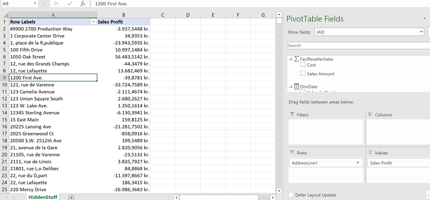
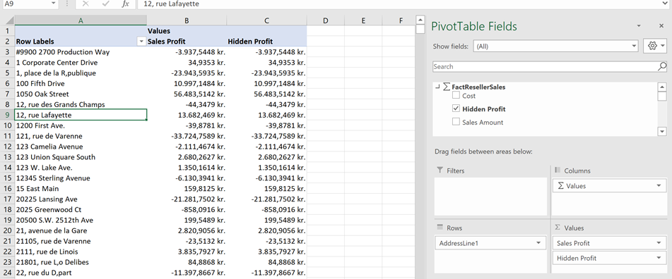
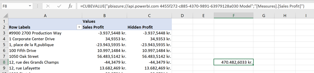
And then we can start analyzing the data in a pivottable

 

Or in PowerView in Excel

 

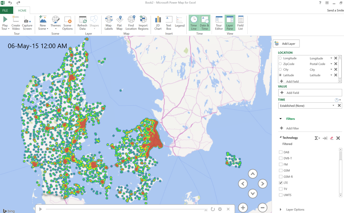
Here is the scary scenario for men when turning 70 …. Looks very dangerous. And Power Map lets us plot by county easily.

 

Or use the new PowerMap filter function to create a heatmap of the regions with 0-3 year old

 

If you sell diapers or sell children’s shoes in Sweden, you can see where to focus.

You can download a copy of the workbook – from here, and let me know if you have questions or like it.