#PowerQuery – Replicate doing an Excel VLOOKUP in M

Power Query has a lot of built in functions, but it doesn’t have a function that exactly matches the VLOOKUP in Excel – but by using the M language and other M functions we can certainly replicate some of the VLOOKUP functionality and make an even more flexible lookup function.

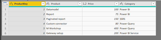
Now the example data is like this

In Excel we would lookup the price for at specific productkey by using this formula

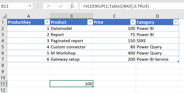
– in this case ProductKey 1 with a price of 100.

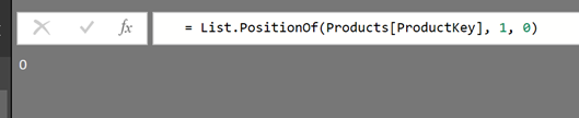
In order to replicate this in Power Query we can use the function List.PositionOf

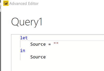
So I add a new blank query

And then use the function List.PositionOf – with the following arguments

List – Is the column ProductKey from my lookuptable Products – refer to like this Products[ProductKey]

Value – Is the value to look in this case the value 1

Occurrence – Is set to 0 to only return one value

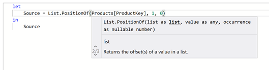
This will return the position of the value in the list – sort of like using the MATCH function in Excel

Now to return the price – we can use this result to lookup the price like this

= Products[Price]{List.PositionOf(Products[ProductKey], 1, 0)}

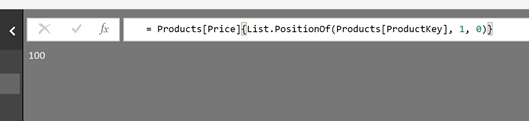
And we get 100 returned which is the price of productkey 1.

The formula is structured like this

=NameOfTheTable[NameOfTheColumnToReturnTheValueOf]{PositionReturnedByListPositionOf}

But we why not change it into a function in PowerQuery so we use the function on all rows in a table or on any table.

The function can be created like this

The code

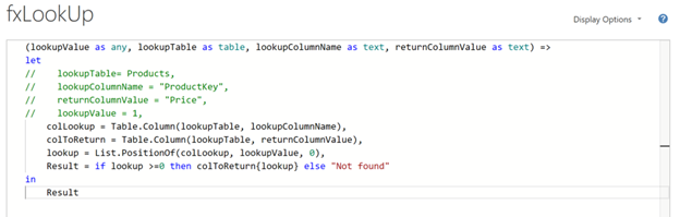
(lookupValue as any, lookupTable as table, lookupColumnName as text, returnColumnValue as text) =>
let
// lookupTable= Products,
// lookupColumnName = "ProductKey",
// returnColumnValue = "Price",
// lookupValue = 1,
 colLookup = Table.Column(lookupTable, lookupColumnName),
 colToReturn = Table.Column(lookupTable, returnColumnValue),
 lookup = List.PositionOf(colLookup, lookupValue, 0),
 Result = if lookup >=0 then colToReturn{lookup} else "Not found"
in
 Result

The function takes 4 arguments –

lookupValue – The value to find – can be any type

lookupTable – The Table/Query to lookup in

lookupColumnName – The name of the column to lookup the value in

returnColumnValue – The name of the column from the table to return

The colLookup is a variable that uses the function Table.Column to return a list of values in the lookup column.

The colToReturn is a variable that uses the function Table.Column to return a list of values from the values you want to return column.

The lookup variable uses the List.PositionOf to find the position/index of the search value in the lookup column.

Result will use an if statement to test whether a position is found and if so returns the value at the position in the colToReturn list – other wise returns the text “Not Found”.

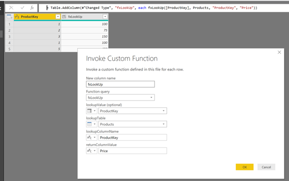
After this we can use the function in other tables to lookup the for instance the Product price like this – by added a invoke Custom Function Column

OBS – I haven’t tried this on a large table so be aware of any performance issues.

Hope you find this useful – and happy Querying

Here is a link to an example file – Link