#PowerBI – Combine visual calculations and numeric parameters to create a dynamic moving average period

With the introduction of visual calculation in the February 2024 release of Power BI desktop (https://powerbi.microsoft.com/en-us/blog/visual-calculations-preview/) – this gives us some new possibilities to add calculations on the individual visual and some new functions gives us some exiciting options.

One example could be to use the MOVINGAVERAGE function (link) to and combine it with numeric range parameter to make it dynamic.

Let me take you through how this can be done

As an example file I have used the datagoblins contoso file sample file that you can download from here (link)

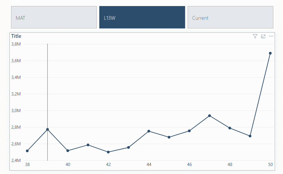
I have added a measure for Sales Value and some time intelligence function to filter the development chart for the selected time intelligence period.

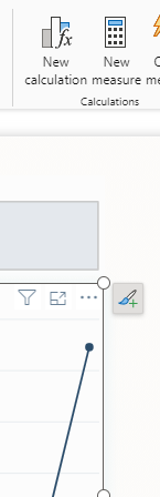
Let’s start by adding a moving average with a visual calculation – If you have enabled the preview feature via options you should see the “New calculation” button enabled in the ribbon.

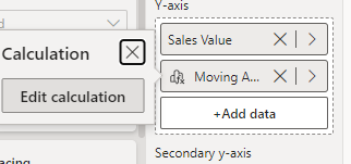
When you click this the Calculation editor will appear

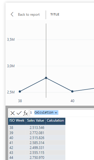
If change the name and click the fx – you can select a template called Moving average

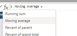
This will add the formula

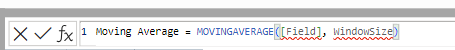
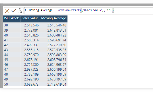
And you can modify it to this

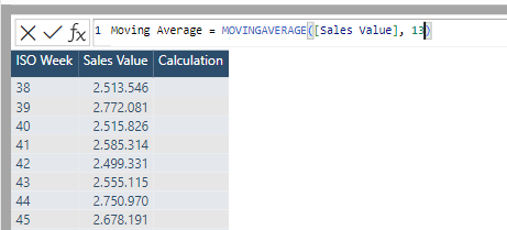
The field refers to the measure you want to calculate the average for and the windowSize refers to the number of rows to include in the calculation. In my example I have week numbers on rows and I want a moving average for the last 13 weeks.

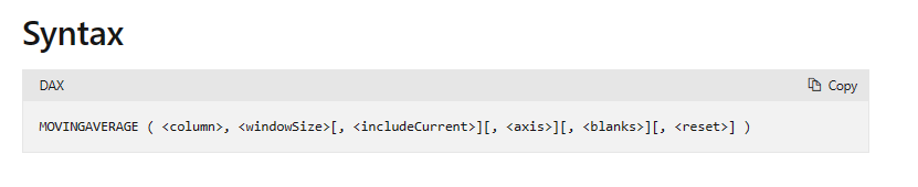
Be aware that the documentation describes the optional arguments as well – click on the image to see the official documentation.

When committing the formula you will see the result

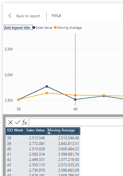
And going back do the report we now have a line showing the moving average for Sales Value for the last 13 weeks … 👍

But what if the user wants a little more control over the length of the period ??

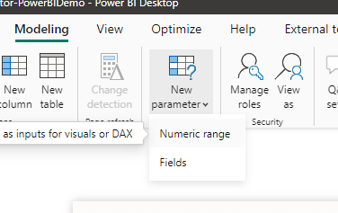
My first thought was – let’s just add a slicer with a numeric range parameter – So I clicked the Numeric range under New Parameter

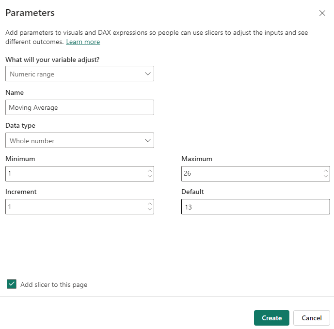
And created it like this

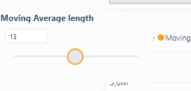
And with some formatting I ended with this slicer

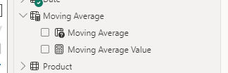
And in the model we can refer to the value of the parameter via created measure “Moving Average Value”

Next step is to modify the visual calculation

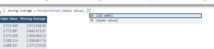
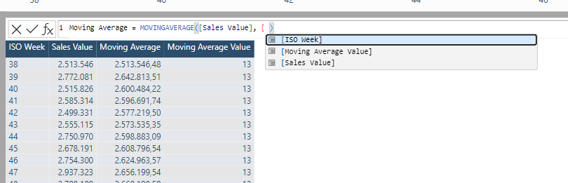
Then I thought lets replace the constant value with the parameter measure value

But in the intellisense I found I couldn’t refer to all measures in the model only the add fields was visible

Okay – lets see if we can cheat – so I added the parameter value field as a tooltip

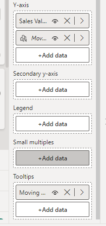
This meant that I was able to refer to it …

But only to be hit be the constraint in the function that the window size must be a constant value

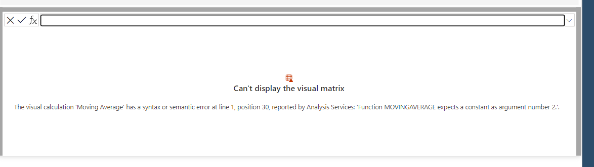
hmmmm… what to do ?? – So I decided to make the solution a bit simpler…

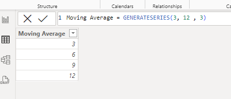
First I changed the parameter table constructor from 1-26

to only 4 different values

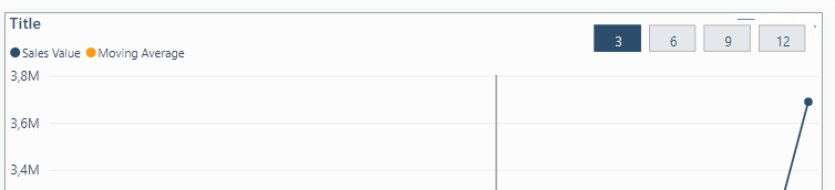
And then modified the slicer to the new slicer and added some formatting and placed it on top of the development chart.

And then I modified the visual calculation to

Moving Average = 
    SWITCH(
        [Moving Average Value],
        3, MOVINGAVERAGE([Sales Value], 3),
        6, MOVINGAVERAGE([Sales Value], 6),
        9, MOVINGAVERAGE([Sales Value], 9),
        12, MOVINGAVERAGE([Sales Value], 12),
        MOVINGAVERAGE([Sales Value], 12)
    )

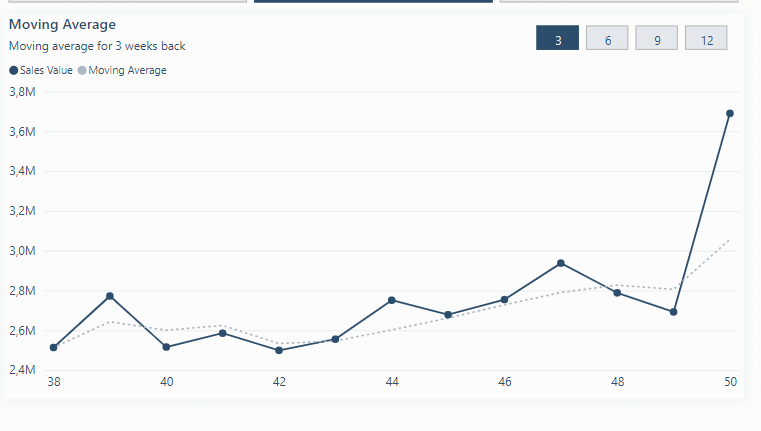
So when ever the user picks another value in the slicer the switch statement will evaluate the current value of the Moving Average Value – and use the appropriate constant value,

And with some further formatting and subtitle we end up with this

You can download the example file from here.

Let me know if you find this useful and/or give the post a like 🙂

Get selected items in a slicer in Excel 2016

My most popular post so far has been “How to get selected items in a slicer without VBA” – Link – and after reading Chris Web’s post about the new Excel 2016 ConcatenateX function in DAX – link – I thought that this function could be used to calculate the selected items in a slicer as well.

And it turned out the function is the perfect solution to do this – and very easy to implement

First I created two simple tables – one with sales and one product table

Add it to the data model via the PowerPivot tab – and I add a calculated measure Sales Value as SUM([SalesValue]).

Now Add a Pivottable and a slicer to filter the table by Product.

Now I add a calculated measure to calculate the selected items

Adding the measure to the pivottable will result in this

But you might want it as a measure in the pivottable but the value stated in a single cell.

This can be done by using the CUBE functions – Use the following formula to accomplish this

=CUBEVALUE(“ThisWorkbookDataModel”,”[Measures].[Selected Products]”,Slicer_Product)

The two member expressions in the formula refers to the measure and then the name of the slicer.

It has never been easier to retrieve the selected items from the slicers with the new CONCATENATEX function..

You can download the example file here